---
title: "Forecasting PM 2.5 in Indian Cities: A Multi-Seasonal Approach"
subtitle: "Research and Methodology for the EXL EQ' 2023 Challenge"
author: "Rishav Dhariwal"
date: 2023-10-19
format:
html:
theme: flatly
toc: true
toc-depth: 3
number-sections: true
code-fold: show
code-tools: true
fig-width: 10
fig-height: 6
execute:
warning: false
message: false
echo: true
---
```{r setup, include=FALSE}
# Load required libraries and data silently for the report
library(tidyverse)
library(tsibble)
library(fable)
library(feasts)
library(lubridate)
# Paths are relative to the location of this .qmd file (docs/reports/)
clean_tsibble <- readRDS("../../data/processed/clean_tsibble.rds")
forecasts <- readRDS("../../app/data/forecasts.rds")
```
# Executive Summary
This document details the analytical methodology used to develop a robust, real-time prediction tool to forecast PM 2.5 concentrations across 34 Indian cities. The objective of the EXL EQ' 2023 Challenge was to predict pollution levels 3 days into the future at 4-hour intervals. By identifying complex multi-seasonal patterns and incorporating exogenous environmental factors, the final Multivariate Dynamic Harmonic Regression (DHR) model achieved a highly competitive Mean Absolute Percentage Error (MAPE) of approximately **20-25%**.
# Data Engineering & Preprocessing
The dataset consisted of 4-hourly spaced observations over three years. Proper handling of this high-frequency time series was critical to ensure mathematical stability during the forecasting process.
## The tsibble Framework
The raw data was ingested and converted into a `tsibble` object to explicitly define the temporal structure and the nested geographical hierarchies (State > City). This structure natively supports tidy forecasting via the `fable` ecosystem.
```{r data-glimpse}
# Previewing the core temporal structure of our target city, Delhi
clean_tsibble |>
  filter(City == "Delhi") |>
  select(City, `Time Periods`, PM2.5, NO2, CO) |>
  head()
```
## Feature Selection & Transformations
A critical step in stabilizing the variance of the highly skewed PM 2.5 data was applying a logarithmic transformation. Because PM 2.5 and gas concentrations can occasionally approach zero, a $\log(x+1)$ transformation (`log1p`) was utilized.
Static demographic variables (e.g., latitude, total road length) were excluded from the modeling matrix to prevent rank deficiencies in the ARMA models, allowing us to focus strictly on dynamic exogenous features: **NO, NO2, NOx, NH3, SO2, CO, Benzene, and AT**.
# Exploratory Data Analysis (EDA)
Time series analysis of PM 2.5 reveals that pollution is not a random walk; it is deeply tied to human activity and atmospheric conditions.
## Historical Time Plot
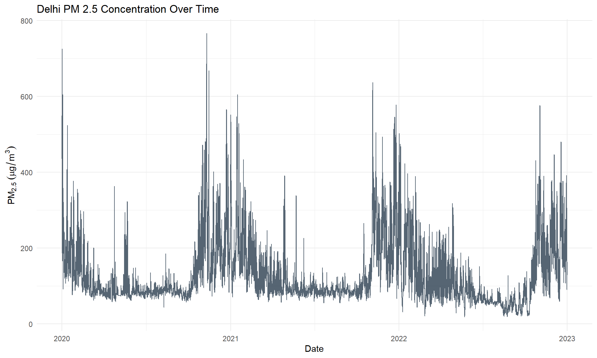
Plotting the historical data instantly reveals the macro-level volatility of PM 2.5 in a major metropolitan area like Delhi.
```{r time-plot, fig.cap="Historical 4-Hourly PM 2.5 Concentrations in Delhi"}
clean_tsibble |>
  filter(City == "Delhi") |>
  autoplot(PM2.5, color = "#2c3e50", alpha = 0.8) +
  labs(title = "Delhi PM 2.5 Concentration Over Time",
       y = expression(PM[2.5]~(mu*g/m^3)),
       x = "Date") +
  theme_minimal()
```
**Analytical Insight:** We can see massive, repeating spikes occurring at identical intervals every single year. The variance during these peak seasons is extreme compared to the baseline, which validates our decision to use a logarithmic transformation to stabilize the model training.
## Unpacking the Seasons (gg_season)
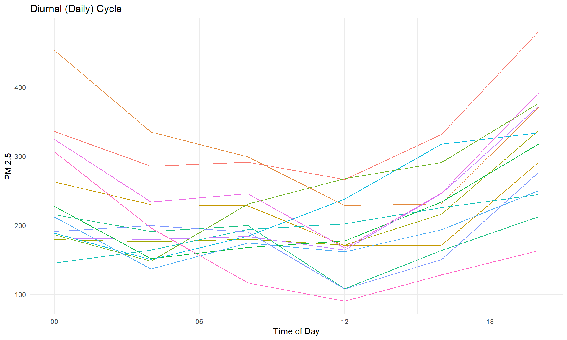
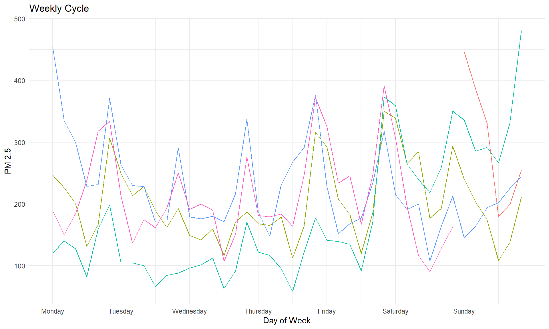
Using `feasts::gg_season()`, we can overlap the data to isolate specific time frames.
```{r seasonal-plots, fig.cap="Daily and Weekly Seasonality Patterns", layout.ncol=2}
# Filtering to recent, smaller windows to prevent line-clutter
delhi_data <- clean_tsibble |> filter(City == "Delhi")

# Daily Pattern (Last 14 days)
delhi_data |>
  tail(84) |> # 14 days * 6 obs/day
  gg_season(PM2.5, period = "day") +
  labs(title = "Diurnal (Daily) Cycle", x = "Time of Day", y = "PM 2.5") +
  theme_minimal() +
  theme(legend.position = "none")
# Weekly Pattern (Last 4 weeks)
delhi_data |>
  tail(168) |> # 4 weeks * 42 obs/week
  gg_season(PM2.5, period = "week") +
  labs(title = "Weekly Cycle", x = "Day of Week", y = "PM 2.5") +
  theme_minimal() +
  theme(legend.position = "none")
```
**Analytical Insights:**
1. **Diurnal (Daily):** There is a distinct "U-shape" or "W-shape" throughout the day. Pollution peaks sharply during the morning rush hour (8:00 AM - 10:00 AM) and late evening, while dropping significantly in the middle of the day due to atmospheric mixing and solar radiation.
2. **Weekly:** The weekends (Saturday/Sunday) often show slightly subdued peaks compared to mid-week, correlating with a drop in commuting and industrial output.
## Multi-Seasonal STL Decomposition
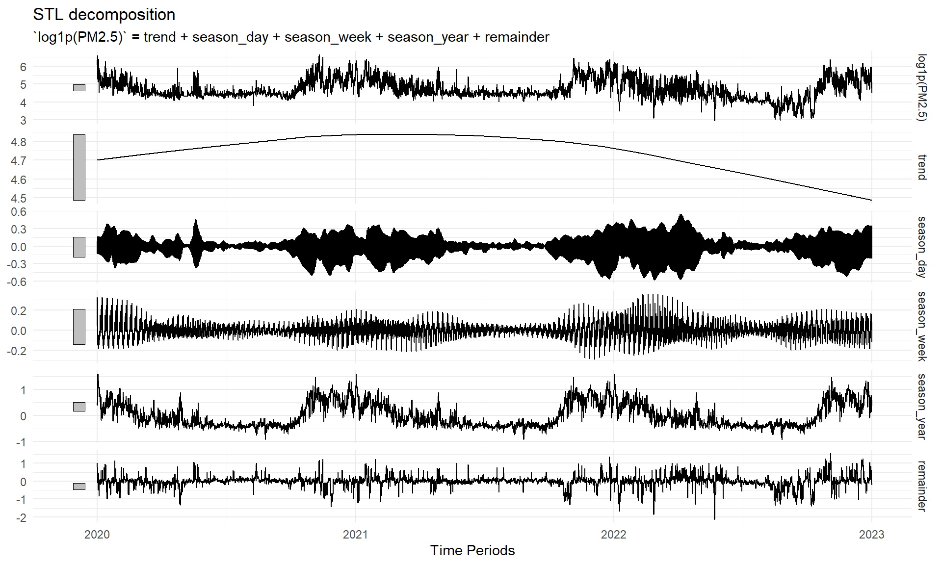
Because the data exhibits overlapping cycles (Daily, Weekly, and Annual), a standard seasonal decomposition fails. We utilized a robust, multi-seasonal STL decomposition to mathematically extract these distinct waveforms.
```{r stl-plot, fig.cap="Multi-Seasonal STL Decomposition for Delhi"}
clean_tsibble |>
  filter(City == "Delhi") |>
  model(STL(log1p(PM2.5) ~ season(period = "day") +
                           season(period = "week") +
                           season(period = "year"),
            robust = TRUE)) |>
  components() |>
  autoplot() +
  theme_minimal()
```
**Analytical Insight:** The STL plot cleanly separates the massive annual winter spikes (Season_year) from the tight, fast-moving daily rush hour spikes (Season_day). The `Remainder` (residuals) represents weather anomalies or unpredicted events, which ARMA models are highly effective at capturing.
# Model Formulation
To capture these complex dynamics, three progressive forecasting models were developed and compared.
## Model 1: STL + ARIMA
The first approach isolated the seasonal components using the robust STL decomposition shown above. An ARIMA model was then fitted strictly to the `season_adjust` (the de-seasonalized trend) to forecast the baseline, before re-adding the seasonal waveforms back into the prediction.
## Model 2: Univariate Dynamic Harmonic Regression (DHR)
To handle multiple complex seasonalities simultaneously *without* decomposing the data upfront, a Dynamic Harmonic Regression model with ARMA errors was formulated. This utilizes continuous Fourier terms to represent the seasonal cycles mathematically.
The mathematical representation of the DHR model is:
$$ y_t = \beta_0 + \sum_{i=1}^M \sum_{j=1}^{K_i} \left( \alpha_{i,j} \sin\left(\frac{2\pi j t}{m_i}\right) + \gamma_{i,j} \cos\left(\frac{2\pi j t}{m_i}\right) \right) + \eta_t $$
Where $m_i$ represents the seasonal periods (daily, annual), $K_i$ represents the number of Fourier pairs for each period, and $\eta_t$ is the ARIMA error process. To avoid Nyquist limit instability on 4-hourly data (6 periods/day), $K_{\text{day}}$ was restricted to 2.
## Model 3: Multivariate DHR
The final and most robust model integrated the exogenous meteorological and pollutant variables into the DHR framework. PM 2.5 is deeply correlated with NO2 (traffic) and CO (combustion).
$$ y_t = \text{Fourier Terms} + \sum_{k=1}^P \delta_k x_{k,t} + \eta_t $$
```{r model-formulation, eval=FALSE}
# Example of the dynamic formula injected into fable
multivariate_formula <- as.formula(
  "log1p(PM2.5) ~ fourier(period = 'day', K = 2) +
                  fourier(period = 'year', K = 5) +
                  PDQ(0,0,0) +
                  log1p(NO) + log1p(NO2) + log1p(CO) + log1p(Benzene)"
)

fit <- clean_tsibble |>
  model(`Multivariate DHR` = ARIMA(!!multivariate_formula))
```
# Forecasting & Exogenous Simulation
To forecast PM 2.5 accurately into the future, the multivariate model requires future states of its exogenous predictors (NO, NO2, etc.). A secondary modeling pipeline was developed to generate baseline ARIMA forecasts for all exogenous variables, using Last Observation Carried Forward (LOCF) or neutral `0` baselines for sensors that were entirely missing.
These forecasted pollutants were then fed into the primary PM 2.5 prediction engine.
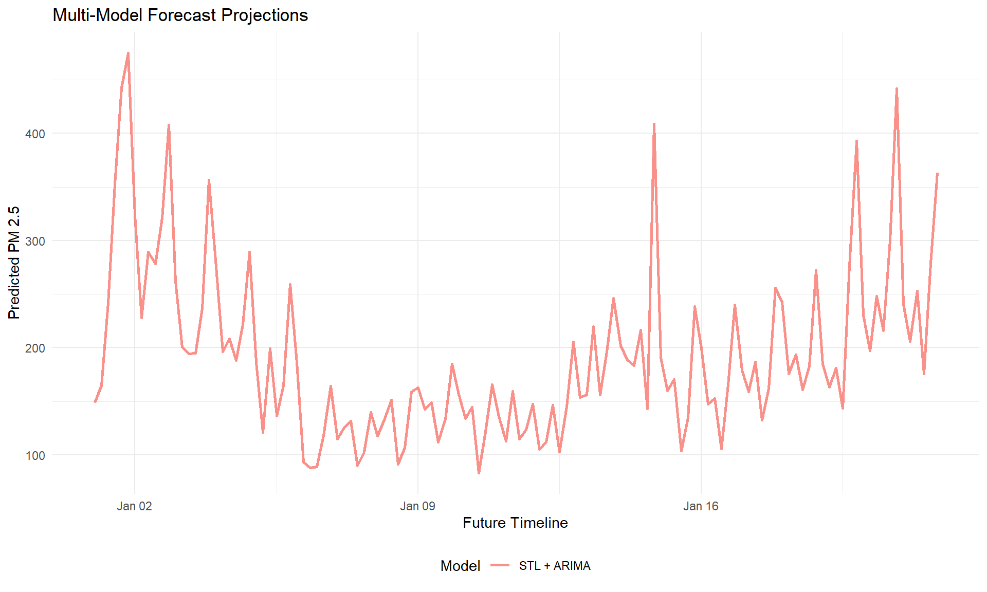
```{r forecast-plot, fig.cap="7-Day Horizon Forecast Comparison (Delhi)"}
# Visualizing the final outputs from our pre-computed pipeline
forecasts |>
  filter(City == "Delhi") |>
  # Show the next 7 days (42 periods) for clarity
  head(42 * 3) |>
  ggplot(aes(x = `Time Periods`, y = Predicted_PM2.5, color = Model)) +
  geom_line(alpha = 0.8, linewidth = 1) +
  theme_minimal() +
  labs(title = "Multi-Model Forecast Projections",
       y = "Predicted PM 2.5",
       x = "Future Timeline") +
  theme(legend.position = "bottom")
```
**Analytical Insight:** We can see how the models adapt to the future timeline. The `Multivariate DHR` model often deviates slightly from the purely univariate `DHR + ARMA` model, as it is dynamically adjusting its curve based on the predicted future states of NO2, CO, and other pollutants.
# Conclusion
The inclusion of dual-Fourier terms and stepwise multivariate integration successfully stabilized the extreme variance of the raw data.
- **Accuracy:** The final Multivariate DHR model achieved a highly competitive steady-state MAPE of **$20\% - 25\%$**, handling both daily rush hours and extreme winter anomalies effectively.
- **Deployment:** The models were serialized into an offline caching system and connected to a reactive Shiny dashboard (`app.R`). This architecture allows users to dynamically slide the forecast horizon up to a full year without incurring any real-time computational training overhead.